Module 1: The Basics of Forward Mode
I. Introduction
Differentiation is fundamental to computational science and is important in many applications, including optimization, sensitivity analysis, and solving differential equations. To be useful in these applications, derivatives must be computed both precisely and efficiently.
Automatic differentiation, sometimes also called algorithmic differentiation or computational differentiation, can efficiently compute derivatives to machine precision, distinguishing itself from both numerical differentiation and symbolic differentiation. To kick things off, we will discuss the differences between automatic differentiation vs. numerical and symbolic differentiation.
Automatic differentiation is not numerical differentiation.
Numerical differentiation refers to a class of methods that computes derivatives through finite difference formulae based on the definition of the derivative,
Such methods are limited in precision due to truncation and roundoff errors because accuracy depends on choosing an appropriate step size h. Let’s consider a basic example.
Demo 1: Errors in The Finite Difference Method
Let’s consider the function \(f(x) = x-\exp(-2\sin^2(4x))\). Using our basic differentiation rules, we can compute the derivative symbolically,
Let’s write some code to calculate derivatives using the finite difference method for this function.
#define our function
def f(x):
    return x-np.exp(-2*np.sin(4*x)**2)

#explicitly define the derivative to compare accuracy
def dfdx(x):
    return 1+16*np.exp(-2*np.sin(4*x)**2)*np.sin(4*x)*np.cos(4*x)

#get numerical derivative at x for stepsize h
def finite_diff(f, x, h):
    return (f(x+h)-f(x))/h

#explore accuracy when changing h
x = np.linspace(0, 2, 1000)
hs = np.logspace(-13, 1, 1000)

errs = np.zeros(len(hs))

for i, h in enumerate(hs):
    err = finite_diff(f, x, h)-dfdx(x) # compute error at each domain point
    errs[i] = np.linalg.norm(err) # store L2 norm of error

#make plot of the error
fig, ax = plt.subplots(1,1, figsize=(10,6))
ax.plot(hs, errs, lw=3)
ax.set_xscale('log')
ax.set_yscale('log')
ax.set_xlabel('h', fontsize=24)
ax.set_ylabel(r'$\|f^{\prime}_{FD}-f^{\prime}_{exact}\|_{L_2}$')
ax.tick_params(labelsize=24)
plt.tight_layout()
The code above produces the following plot, showing the effects of the choice of h on the accuracy of the finite difference method.
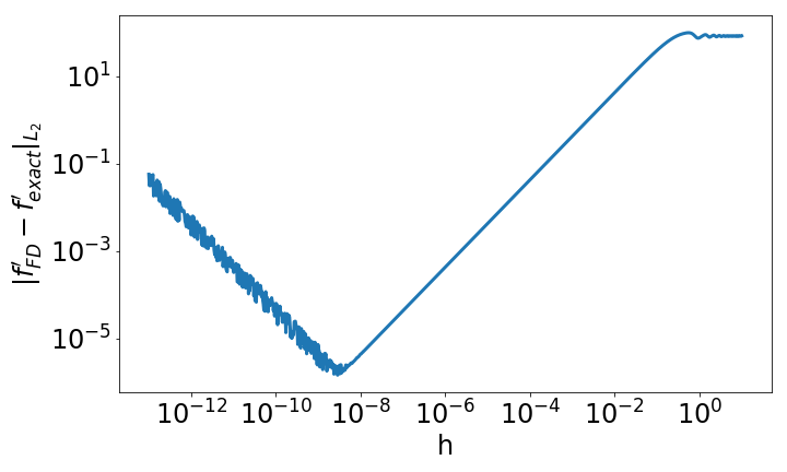
In the plot above, we see that the accuracy of the derivative calculation is highly dependent on our choice of h. When we choose h too large, the numerical approximation is no longer accurate, but for h too small, we begin to see round off errors from limitations in machine precision. We can do a back of the envelope calculation to see the main idea in action. Say you choose \(h = 10^{-12}\), which isn’t machine precision, but it’s pretty close. Now, the numerator of the finite difference formula is f(x + h) - f(x). The smallest this difference could be would be machine precision, \(h_m \approx 10^{-16}\), due to floating point errors. Suppose this is the case. Then, when dividing that difference by the selected h, there is an error of \(10^{-4}\)! This is pretty far away from machine precision and it happened because h is too small.
Check out Exercise 1 for another example motivating the use of automatic differentiation.
Automatic differentiation is not symbolic differentiation.
Symbolic differentiation computes exact expressions for derivatives using expression trees. As seen in the function in Demo 1, exact expressions for derivatives can quickly become complex, which can sometimes make computing derivatives in this manner computationally inefficient.
Now, to summarize what we have learned so far:
Automatic differentiation is a procedure that computes derivatives to machine precision without explicitly forming an expression for the derivative. It relies on application of the ideas of the chain rule to decompose complex functions into elementary functions for which we can compute the derivative exactly.
Automatic differentiation can be split into two primary “modes”: forward and reverse. Both modes allow for efficient and accurate computation of derivatives. Advanced approaches exist for combining forward and reverse mode into a hybrid, but these are beyond the scope of these introductory modules.
The properties of automatic differentiation make it useful for a variety of applications including machine learning, parameter optimization, sensitivity analysis, physical modeling, and probabilistic inference. In the rest of this module, we will begin to explore the mechanics of automatic differentiation.
II. The Basics of Forward Mode
Automatic differentiation is something of a compromise between numerical differentiation and symbolic differentiation. Automatic differentiation provides numerical values of the derivatives of a function. These numerical values are correct to machine precision and are not influenced by any kind of “step size” like in numerical differentiation. Even though automatic differentiation provides derivatives to machine precision, it does not require evaluation of a symbolic derivative.
One other thing to keep in mind about automatic differentation is that we usually think of it as yielding the derivative of a function evaluated at a specific point. This should be borne in mind throughout this module. We will evaluate a function at a specific point and we will automatically get its derivative at that same point.
The major concept underlying automatic differentiation is the chain rule. Recall from calculus that the chain rule states that to find the derivative of a composition of functions, we multiply a series of derivatives. For illustration, let \(f(t) = g(h(t))\). We have
This can be generalized to functions of multiple inputs, which we will discuss in more detail in Module 2.
Elementary Functions
Every function can be decomposed into a set of binary elementary operations or unary elementary functions. Elementary operations include addition, subtraction, multiplication, division, and exponentiation. Elementary functions include the natural exponential and natural logarithm, trigonometric functions, and polynomials. The sigmoid function and the hyperbolic trigonometric functions can also be considered elementary functions, though they can be formed from the natural exponential.
Basic calculus provides closed form differentiation rules for these elementary functions. This means that we can compose these functions to form more complex functions and find the derivative of these more complex functions using the chain rule. This is the key idea behind automatic differentiation. We know the derivatives of the elementary functions. Complicated functions are composed of elementary functions. The chain rule provides a route to calculating derivatives of functions that are composed of other functions.
To understand this composition of elementary functions, we can think of the composition of functions as having an underlying graph structure. You will learn much more about this graph structure in Module 2, including a way to build it by hand. For now, you will practice visualizing the graph with a special tool.
III. A Tool for Visualizing Automatic Differentiation
The Auto-eD tool is a pedagogical tool to help visualize the processes underlying automatic differentiation. In particular, this tool allows us to visualize the underlying graph structure of a calculation when decomposed into elementary functions. In addition to helping to visualize this graph, the tool can also be used to view the computational traces that occur at each node of the graph. These ideas will be discussed much more in Module 2.
Auto-eD Web Application
The tool can be accessed directly through a web browser:
This option is good for people who want to explore automatic differentiation.
Developer Instructions
Auto-eD is open source. You are free to check out the code and even contribute improvements. To run the tool with the ability to modify and contribute to the code, you may choose to clone the Github repo to have direct access to the code for the web app and access to the underlying package. From the terminal,
1. Clone the repo:
git clone https:github.com/lindseysbrown/Auto-eD
2. Install the dependencies:
pip install -r requirements.txt
3. Launch the web app from the terminal:
python ADapp.py
Visit http://0.0.0.0:5000 to use the tool through your local server.
We welcome improvements and contributions! You can find more details about the underlying package in the DeveloperDocumentation.ipynb. If you would like to contribute to this project, please follow these steps:
Clone the repo
Create a new branch with an informative branch name
Make sure all your updates are on the new branch
Make a pull request to master branch and wait for the core developers to respond!
IV. A First Demo of Automatic Differentiation
Let’s use the Auto-eD web application tool to visualize the function from Demo 1. Our function of interest is: \(f(x) = x-\exp(-2\sin^2(4x))\).
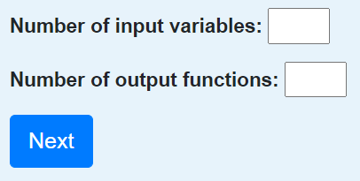
The function has a single input variable (x), so just enter 1 in the “Number of input variables” field.
Our function is scalar valued, so we enter that our function has 1 output.
3. Use the calculator interface to enter our function. (Click on the “<-” button or the “Clear All” button to correct the function if you make a mistake.) With the current release, you must click on the function buttons on the calculator rather than typing them from the keyboard.
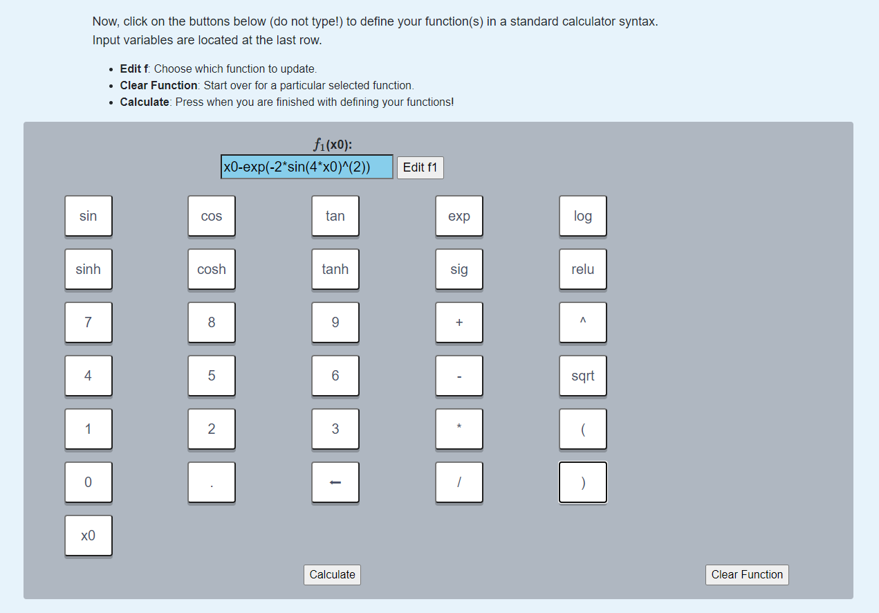
4. Press the “Calculate” button. This will bring you to the next page with options to help you visualize both the forward and reverse mode of automatic differentiation.
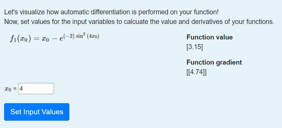
5. Enter the value for x at which you’d like to evaluate the function. For the purposes of this demo, we’ll choose x=4. Click the “Set Input Values” button.
Note that automatic differentiation yields the value of the derivative at a specific point. It does not compute a symbolic expression for the derivative.
You’ll see the values for the function and derivative appear beside your function and input values you selected.
7. Below this, you’ll see buttons for which function you’d like to visualize. In this example, we only have a single function, so click on “f1” button.
8. This will generate the computational graph for both forward and reverse mode as well as the computational trace table. We’ll talk more about the computational table and reverse mode in the next modules, so for now let’s just focus on the computational graph in forward mode.
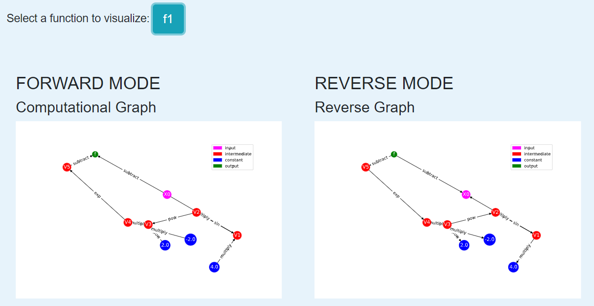
9. The single magenta node represents the input to the function. The single green output node represents the output value of our function. The red nodes represent intermediate function values. Notice that all of the nodes are connected by elementary operations on the labelled edges.
(Hint: Occasionally the graphs may be difficult to read depending on the complexity of the function that you are visualizing. You can try running the tool a second time to get a different configuration of the nodes. Alternatively, for large functions, you can run the package from the command line, which will generate graphs that you can maximize to resize the edges.)
Some Key Takeaways
Our function was decomposed into a series of elementary operations.
These operations include both basic binary operations (addition, subtraction, multiplication, and division), unary operations (negation), and elementary functions (exponential functions, trigonometric functions).
Using this graph to compute the derivative is the same process as using the chain rule to compute the derivative, allowing the derivative to be computed to machine precision.
Don’t worry if you don’t understand this perfectly yet. At this time, you should appreciate that automatic differentiation gives the exact value of the derivative at a specified point. The graph displayed by the tool is a representation of the function itself and depicts how the function is built up from elementary functions.
V. Exercises
Exercise 1: Motivating Automatic Differentiation
Write a Python function that takes two inputs: 1. a function (of a single variable) and 2. a value of \(h\). This function should return a function which has a single input: a value of \(x\). This inner function should compute the numerical approximation of the derivative of \(f\) with stepsize \(h\) at \(x\).
Note: This part of the exercise is meant to be implemented as a closure in Python. It consists of an outer function and an inner function.
Let \(f(x) = ln(x)\). For \(0.2\leq x \leq 0.4\), make a plot comparing the numerically estimated derivative for \(h=10^{-1}, h=10^{-7}\), and \(h=10^{-15}\) to the analytic derivative (which should be used explicitly).
Note: All plots should be on the same figure. This means there should be 4 lines: three for the different values of \(h\) and one for the true solution. Make sure to include a legend and that the different lines are distinguishable.
Answer the following questions:
Which value of \(h\) most closely approximates the true derivative? What happens for values of \(h\) that are too small? What happens for values of \(h\) that are too large?
How does automatic differentiation address these problems?
Exercise 2: Basic Graph Structure of Calculations
Consider the function \(f(x)= \tan(x^2+3)+x\).
Draw the graph with the visualization tool.
Exercise 3: Looking Toward Multiple Inputs
We can use the same process to compute derivatives for functions of multiple inputs. Consider the function:
Practice drawing the computational graph for this function using the Auto-eD visualization tool. We’ll discuss the theory behind functions of multiple inputs in the next module.